Understanding Partial Updates


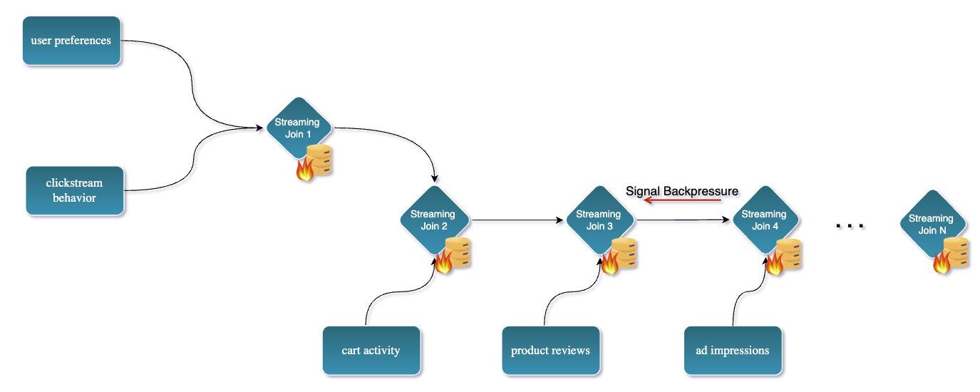
Traditional streaming data pipelines often need to join many tables or streams on a primary key to create a wide view. For example, imagine you’re building a real-time recommendation engine for an e-commerce platform. To serve highly personalized recommendations, your system needs a complete 360° view of each user, including: user preferences, past purchases, clickstream behavior, cart activity, product reviews, support tickets, ad impressions, and loyalty status.
That’s at least 8 different data sources, each producing updates independently.
Joining multiple data streams at scale, although it works with Apache Flink it can be really challenging and resource-intensive. More specifically, it can lead to:
- Really large state sizes in Flink: as it needs to buffer all incoming events until they can be joined. In many case states need to be kept around for a long period of time if not indefinitely.
- Deal with checkpoints overhead and backpressure: as the join operation and large state uploading can create a bottleneck in the pipeline.
- States are not easy to inspect and debug: as they are often large and complex. This can make it difficult to understand what is happening in the pipeline and why certain events are not being processed correctly.
- State TTL can lead to inconsistent results: as events may be dropped before they can be joined. This can lead to data loss and incorrect results in the final output.
Overall, this approach not only consumes a lot of memory and CPU, but also complicates the job design and maintenance.
Partial Updates: A Different Approach with Fluss
Fluss introduces a more elegant solution: partial updates on a primary key table.
Instead of performing multi-way joins in the streaming job, Fluss allows each data stream source to independently update only its relevant columns into a shared wide table identified by the primary key.
In Fluss, you can define a wide table (for example, a user_profile table based on a user_id) that contains all possible fields from all sources.
Each source stream then writes partial rows – only the fields it knows about – into this table.
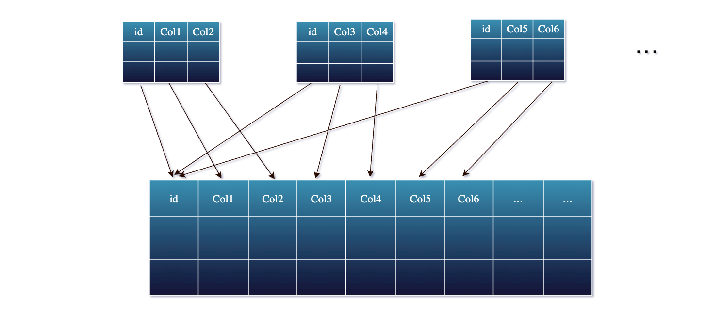
Fluss’s storage engine automatically merges these partial updates together based on the primary key. Essentially, Fluss maintains the latest combined value for each key, so you don’t have to manage large join states in Flink.
Under the hood, when a new partial update for a key arrives, Fluss will look up the existing record for that primary key, update the specific columns provided, and leave other columns unchanged. The result is written back as the new version of the record. This happens in real-time, so the table is always up-to-date with the latest information from all streams.
Next, let's try and better understand how this works in practice with a concrete example.
Example: Building a Unified Wide Table
You can find the full source code on github here.
Start by cloning the repository, run docker compose up to spin up the development enviroment and finally grab a terminal
into the jobmanager and start the Flink SQL cli, by running the following command:
./bin/sql-client.sh
Great so far ! 👍
Step 1: The first thing we need to do is to create a Flink catalog that will be used to store the tables we are going to create.
Let's create a catalog called fluss_catalog and use this catalog.
CREATE CATALOG fluss_catalog WITH (
    'type' = 'fluss',
    'bootstrap.servers' = 'coordinator-server:9123'
);

USE CATALOG fluss_catalog;
Step 2: Then let's create 3 tables to represent the different data sources that will be used to build the recommendations wide table.
-- Recommendations – model scores
CREATE TABLE recommendations (
    user_id  STRING,
    item_id  STRING,
    rec_score DOUBLE,
    rec_ts   TIMESTAMP(3),
    PRIMARY KEY (user_id, item_id) NOT ENFORCED
) WITH ('bucket.num' = '3', 'table.datalake.enabled' = 'true');


-- Impressions – how often we showed something
CREATE TABLE impressions (
    user_id STRING,
    item_id STRING,
    imp_cnt INT,
    imp_ts  TIMESTAMP(3),
    PRIMARY KEY (user_id, item_id) NOT ENFORCED
) WITH ('bucket.num' = '3', 'table.datalake.enabled' = 'true');

-- Clicks – user engagement
CREATE TABLE clicks (
    user_id  STRING,
    item_id  STRING,
    click_cnt INT,
    clk_ts    TIMESTAMP(3),
    PRIMARY KEY (user_id, item_id) NOT ENFORCED
) WITH ('bucket.num' = '3', 'table.datalake.enabled' = 'true');

CREATE TABLE user_rec_wide (
    user_id   STRING,
    item_id   STRING,
    rec_score DOUBLE,   -- updated by recs stream
    imp_cnt   INT,      -- updated by impressions stream
    click_cnt INT,      -- updated by clicks stream
    PRIMARY KEY (user_id, item_id) NOT ENFORCED
) WITH ('bucket.num' = '3', 'table.datalake.enabled' = 'true');
Step 3: Of course, we will need some sample data to work with , so let's go on and insert some records into the tables. 💻
-- Recommendations – model scores
INSERT INTO recommendations VALUES
    ('user_101','prod_501',0.92 , TIMESTAMP '2025-05-16 09:15:02'),
    ('user_101','prod_502',0.78 , TIMESTAMP '2025-05-16 09:15:05'),
    ('user_102','prod_503',0.83 , TIMESTAMP '2025-05-16 09:16:00'),
    ('user_103','prod_501',0.67 , TIMESTAMP '2025-05-16 09:16:20'),
    ('user_104','prod_504',0.88 , TIMESTAMP '2025-05-16 09:16:45');
-- Impressions – how often each (user,item) was shown
INSERT INTO impressions VALUES
    ('user_101','prod_501', 3, TIMESTAMP '2025-05-16 09:17:10'),
    ('user_101','prod_502', 1, TIMESTAMP '2025-05-16 09:17:15'),
    ('user_102','prod_503', 7, TIMESTAMP '2025-05-16 09:18:22'),
    ('user_103','prod_501', 4, TIMESTAMP '2025-05-16 09:18:30'),
    ('user_104','prod_504', 2, TIMESTAMP '2025-05-16 09:18:55');
-- Clicks – user engagement
INSERT INTO clicks VALUES
    ('user_101','prod_501', 1, TIMESTAMP '2025-05-16 09:19:00'),
    ('user_101','prod_502', 2, TIMESTAMP '2025-05-16 09:19:07'),
    ('user_102','prod_503', 1, TIMESTAMP '2025-05-16 09:19:12'),
    ('user_103','prod_501', 1, TIMESTAMP '2025-05-16 09:19:20'),
    ('user_104','prod_504', 1, TIMESTAMP '2025-05-16 09:19:25');
Note: 🚨 So far the jobs we run were bounded jobs, so they will finish after inserting the records. Moving forward we will run some streaming jobs. So keep in mind that each job runs with a
parallelism of 3and our environment is set upwith 10 slots total. So make sure to keep an eye to the Flink Web UI to see how many slots are used and how many are available and stop some jobs when are no longer needed to free up resourecs.
Step 4: At this point let's open up a separate terminal and start the Flink SQL CLI.
In this new terminal, make sure to run set the result-mode:
SET 'sql-client.execution.result-mode' = 'tableau';
and then run:
SELECT * FROM user_rec_wide;
to observe the output of the table, as we insert partially records into the it from the different sources.
Step 5: Let's insert the records from the recommendations table into the user_rec_wide table.
-- Apply recommendation scores
INSERT INTO user_rec_wide (user_id, item_id, rec_score)
SELECT
    user_id,
    item_id,
    rec_score
FROM recommendations;
Output: Notice, how only the related columns are updated in the user_rec_wide table and the rest of the columns are NULL.
Flink SQL> SELECT * FROM user_rec_wide;
+----+--------------------------------+--------------------------------+--------------------------------+-------------+-------------+
| op |                        user_id |                        item_id |                      rec_score |     imp_cnt |   click_cnt |
+----+--------------------------------+--------------------------------+--------------------------------+-------------+-------------+
| +I |                       user_101 |                       prod_501 |                           0.92 |      <NULL> |      <NULL> |
| +I |                       user_101 |                       prod_502 |                           0.78 |      <NULL> |      <NULL> |
| +I |                       user_104 |                       prod_504 |                           0.88 |      <NULL> |      <NULL> |
| +I |                       user_102 |                       prod_503 |                           0.83 |      <NULL> |      <NULL> |
| +I |                       user_103 |                       prod_501 |                           0.67 |      <NULL> |      <NULL> |
Step 5: Next, let's insert the records from the impressions table into the user_rec_wide table.
-- Apply impression counts
INSERT INTO user_rec_wide (user_id, item_id, imp_cnt)
SELECT
    user_id,
    item_id,
    imp_cnt
FROM impressions;
Output: Notice how the impressions records are inserted into the user_rec_wide table and the imp_cnt column is updated.
Flink SQL> SELECT * FROM user_rec_wide;
+----+--------------------------------+--------------------------------+--------------------------------+-------------+-------------+
| op |                        user_id |                        item_id |                      rec_score |     imp_cnt |   click_cnt |
+----+--------------------------------+--------------------------------+--------------------------------+-------------+-------------+
| +I |                       user_101 |                       prod_501 |                           0.92 |      <NULL> |      <NULL> |
| +I |                       user_101 |                       prod_502 |                           0.78 |      <NULL> |      <NULL> |
| +I |                       user_104 |                       prod_504 |                           0.88 |      <NULL> |      <NULL> |
| +I |                       user_102 |                       prod_503 |                           0.83 |      <NULL> |      <NULL> |
| +I |                       user_103 |                       prod_501 |                           0.67 |      <NULL> |      <NULL> |


| -U |                       user_101 |                       prod_501 |                           0.92 |      <NULL> |      <NULL> |
| +U |                       user_101 |                       prod_501 |                           0.92 |           3 |      <NULL> |
| -U |                       user_101 |                       prod_502 |                           0.78 |      <NULL> |      <NULL> |
| +U |                       user_101 |                       prod_502 |                           0.78 |           1 |      <NULL> |
| -U |                       user_104 |                       prod_504 |                           0.88 |      <NULL> |      <NULL> |
| +U |                       user_104 |                       prod_504 |                           0.88 |           2 |      <NULL> |
| -U |                       user_102 |                       prod_503 |                           0.83 |      <NULL> |      <NULL> |
| +U |                       user_102 |                       prod_503 |                           0.83 |           7 |      <NULL> |
| -U |                       user_103 |                       prod_501 |                           0.67 |      <NULL> |      <NULL> |
| +U |                       user_103 |                       prod_501 |                           0.67 |           4 |      <NULL> |
Step 6: Finally, let's insert the records from the clicks table into the user_rec_wide table.
-- Apply click counts
INSERT INTO user_rec_wide (user_id, item_id, click_cnt)
SELECT
    user_id,
    item_id,
    click_cnt
FROM clicks;
Output: Notice how the clicks records are inserted into the user_rec_wide table and the click_cnt column is updated.
Flink SQL> SELECT * FROM user_rec_wide;
+----+--------------------------------+--------------------------------+--------------------------------+-------------+-------------+
| op |                        user_id |                        item_id |                      rec_score |     imp_cnt |   click_cnt |
+----+--------------------------------+--------------------------------+--------------------------------+-------------+-------------+
| +I |                       user_101 |                       prod_501 |                           0.92 |      <NULL> |      <NULL> |
| +I |                       user_101 |                       prod_502 |                           0.78 |      <NULL> |      <NULL> |
| +I |                       user_104 |                       prod_504 |                           0.88 |      <NULL> |      <NULL> |
| +I |                       user_102 |                       prod_503 |                           0.83 |      <NULL> |      <NULL> |
| +I |                       user_103 |                       prod_501 |                           0.67 |      <NULL> |      <NULL> |


| -U |                       user_101 |                       prod_501 |                           0.92 |      <NULL> |      <NULL> |
| +U |                       user_101 |                       prod_501 |                           0.92 |           3 |      <NULL> |
| -U |                       user_101 |                       prod_502 |                           0.78 |      <NULL> |      <NULL> |
| +U |                       user_101 |                       prod_502 |                           0.78 |           1 |      <NULL> |
| -U |                       user_104 |                       prod_504 |                           0.88 |      <NULL> |      <NULL> |
| +U |                       user_104 |                       prod_504 |                           0.88 |           2 |      <NULL> |
| -U |                       user_102 |                       prod_503 |                           0.83 |      <NULL> |      <NULL> |
| +U |                       user_102 |                       prod_503 |                           0.83 |           7 |      <NULL> |
| -U |                       user_103 |                       prod_501 |                           0.67 |      <NULL> |      <NULL> |
| +U |                       user_103 |                       prod_501 |                           0.67 |           4 |      <NULL> |


| -U |                       user_103 |                       prod_501 |                           0.67 |           4 |      <NULL> |
| +U |                       user_103 |                       prod_501 |                           0.67 |           4 |           1 |
| -U |                       user_101 |                       prod_501 |                           0.92 |           3 |      <NULL> |
| +U |                       user_101 |                       prod_501 |                           0.92 |           3 |           1 |
| -U |                       user_101 |                       prod_502 |                           0.78 |           1 |      <NULL> |
| +U |                       user_101 |                       prod_502 |                           0.78 |           1 |           2 |
| -U |                       user_104 |                       prod_504 |                           0.88 |           2 |      <NULL> |
| +U |                       user_104 |                       prod_504 |                           0.88 |           2 |           1 |
| -U |                       user_102 |                       prod_503 |                           0.83 |           7 |      <NULL> |
| +U |                       user_102 |                       prod_503 |                           0.83 |           7 |           1 |
Reminder: ‼️As mentioned before make sure to stop the jobs that are no longer needed to free up resources.
Now let's switch to batch mode and query the current snapshot of the user_rec_wide table.
But before that, let's start the Tiering Service that allows offloading the tables as Lakehouse tables.
Step 7: Open a new terminal 💻 in the Coordinator Server and run the following command to start the Tiering Service:
./bin/lakehouse.sh -D flink.rest.address=jobmanager -D flink.rest.port=8081 -D flink.execution.checkpointing.interval=30s -D flink.parallelism.default=2
The configured checkpoint is flink.execution.checkpointing.interval=30s so wait a bit until the first checkpoint is created
and data gets offloading to the Lakehouse tables.
Step 8: Finally let's switch to batch mode and query the current snapshot of the user_rec_wide table.
SET 'execution.runtime-mode' = 'batch';

Flink SQL> SELECT * FROM user_rec_wide;
+----------+----------+-----------+---------+-----------+
|  user_id |  item_id | rec_score | imp_cnt | click_cnt |
+----------+----------+-----------+---------+-----------+
| user_102 | prod_503 |      0.83 |       7 |         1 |
| user_103 | prod_501 |      0.67 |       4 |         1 |
| user_101 | prod_501 |      0.92 |       3 |         1 |
| user_101 | prod_502 |      0.78 |       1 |         2 |
| user_104 | prod_504 |      0.88 |       2 |         1 |
+----------+----------+-----------+---------+-----------+
5 rows in set (2.63 seconds)
🎉 That's it! You have successfully created a unified wide table using partial updates in Fluss.
Conclusion
Partial updates in Fluss enable an alternative approach in how we design streaming data pipelines for enriching or joining data.
When all your sources share a primary key - otherwise you can mix & match streaming lookup joins - you can turn the problem on its head: update a unified table incrementally, rather than joining streams on the fly.
The result is a more scalable, maintainable, and efficient pipeline. Engineers can spend less time wrestling with Flink’s state, checkpoints and join mechanics, and more time delivering fresh, integrated data to power real-time analytics and applications. With Fluss handling the merge logic, achieving a single, up-to-date view from multiple disparate streams becomes way more elegant. 😁
And before you go 😊 don’t forget to give Fluss 🌊 some ❤️ via ⭐ on GitHub